


Some error occured while loading the Quick View. Please close the Quick View and try reloading the page.
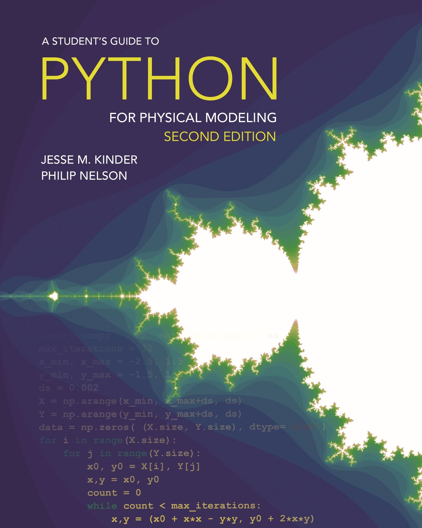
A fully updated tutorial on the basics of the Python programming language for science students
Python is a computer programming language that has gained popularity throughout the sciences. This fully updated second edition of A Student's Guide to Python for Physical Modeling aims to help you, the student, teach yourself enough of the Python programming language to get started with physical modeling. You will learn how to install an open-source Python programming environment and use it to accomplish many common scientific computing tasks: importing, exporting, and visualizing data; numerical analysis; and simulation. No prior programming experience is assumed.
This guide introduces a wide range of useful tools, including:
- Basic Python programming and scripting
- Numerical arrays
- Two- and three-dimensional graphics
- Animation
- Monte Carlo simulations
- Numerical methods, including solving ordinary differential equations
- Image processing
Numerous code samples and exercises—with solutions—illustrate new ideas as they are introduced. This guide also includes supplemental online resources: code samples, data sets, tutorials, and more. This edition includes new material on symbolic calculations with SymPy, an introduction to Python libraries for data science and machine learning (pandas and sklearn), and a primer on Python classes and object-oriented programming. A new appendix also introduces command line tools and version control with Git.

- Let’s Go
- 1 Getting Started with Python
- 1.1 Algorithms and algorithmic thinking
- 1.1.1 Algorithmic thinking
- 1.1.2 States
- 1.1.3 What does a = a + 1 mean?
- 1.1.4 Symbolic versus numerical
- 1.2 Launch Python
- 1.2.1 IPython console
- 1.2.2 Error messages
- 1.2.3 Sources of help
- 1.2.4 Good practice: Keep a log
- 1.3 Python modules
- 1.3.1 import
- 1.3.2 from . . . import
- 1.3.3 NumPy and PyPlot
- 1.4 Python expressions
- 1.4.1 Numbers
- 1.4.2 Arithmetic operations and predefined functions
- 1.4.3 Good practice: Variable names
- 1.4.4 More about functions
- 1.1 Algorithms and algorithmic thinking
- 2 Organizing Data
- 2.1 Objects and their methods
- 2.2 Lists, tuples, and arrays
- 2.2.1 Creating a list or tuple
- 2.2.2 NumPy arrays
- 2.2.3 Filling an array with values
- 2.2.4 Concatenation of arrays
- 2.2.5 Accessing array elements
- 2.2.6 Arrays and assignments
- 2.2.7 Slicing
- 2.2.8 Flattening an array
- 2.2.9 Reshaping an array
- 2.2.10 T2 Lists and arrays as indices
- 2.3 Strings
- 2.3.1 Raw strings
- 2.3.2 Formatting strings with the format ( ) method
- 2.3.3 T2 Formatting strings with %
- 3 Structure and Control
- 3.1 Loops
- 3.1.1 for loops
- 3.1.2 while loops
- 3.1.3 Very long loops
- 3.1.4 Infinite loops
- 3.2 Array operations
- 3.2.1 Vectorizing math
- 3.2.2 Matrix math
- 3.2.3 Reducing an array
- 3.3 Scripts
- 3.3.1 The Editor
- 3.3.2 T2 Other editors
- 3.3.3 First steps to debugging
- 3.3.4 Good practice: Commenting
- 3.3.5 Good practice: Using named parameters
- 3.3.6 Good practice: Units
- 3.4 Contingent behavior: Branching
- 3.4.1 The if statement
- 3.4.2 Testing equality of floats
- 3.5 Nesting
- 3.1 Loops
- 4 Data In, Results Out
- 4.1 Importing data
- 4.1.1 Obtaining data
- 4.1.2 Bringing data into Python
- 4.2 Exporting data
- 4.2.1 Scripts
- 4.2.2 Data files
- 4.3 Visualizing data
- 4.3.1 The plot command and its relatives
- 4.3.2 Log axes
- 4.3.3 Manipulate and embellish
- 4.3.4 Replacing curves
- 4.3.5 T2 More about figures and their axes
- 4.3.6 T2 Error bars
- 4.3.7 3D graphs
- 4.3.8 Multiple plots
- 4.3.9 Subplots
- 4.3.10 Saving figures
- 4.3.11 T2 Using figures in other applications
- 4.1 Importing data
- 5 First Computer Lab
- 5.1 HIV example
- 5.1.1 Explore the model
- 5.1.2 Fit experimental data
- 5.2 Bacterial example
- 5.2.1 Explore the model
- 5.2.2 Fit experimental data
- 5.1 HIV example
- 6 Random Number Generation and Numerical Methods
- 6.1 Writing your own functions
- 6.1.1 Defining functions in Python
- 6.1.2 Updating functions
- 6.1.3 Arguments, keywords, and defaults
- 6.1.4 Return values
- 6.1.5 Functional programming
- 6.2 Random numbers and simulation
- 6.2.1 Simulating coin flips
- 6.2.2 Generating trajectories
- 6.3 Histograms and bar graphs
- 6.3.1 Creating histograms
- 6.3.2 Finer control
- 6.4 Contour plots, surface plots, and heat maps
- 6.4.1 Generating a grid of points
- 6.4.2 Contour plots
- 6.4.3 Surface plots
- 6.4.4 Heat maps
- 6.5 Numerical solution of nonlinear equations
- 6.5.1 General real functions
- 6.5.2 Complex roots of polynomials
- 6.6 Solving systems of linear equations
- 6.7 Numerical integration
- 6.7.1 Integrating a predefined function
- 6.7.2 Integrating your own function
- 6.7.3 Oscillatory integrands
- 6.7.4 T2 Parameter dependence
- 6.8 Numerical solution of differential equations
- 6.8.1 Reformulating the problem
- 6.8.2 Solving an ODE
- 6.8.2 T2 Parameter dependence
- 6.8.4 Other ODE solvers
- 6.9 Vector fields and streamlines
- 6.9.1 Vector fields
- 6.9.2 Streamlines
- 6.1 Writing your own functions
- 7 Second Computer Lab
- 7.1 Generating and plotting trajectories
- 7.2 Plotting the displacement distribution
- 7.3 Rare events
- 7.3.1 The Poisson distribution
- 7.3.2 Waiting times
- 8 Images and Animation
- 8.1 Image processing
- 8.1.1 Images as NumPy arrays
- 8.1.2 Saving and displaying images
- 8.1.3 Manipulating images
- 8.2 Displaying data as an image
- 8.3 Animation
- 8.3.1 Creating animations
- 8.3.2 Saving animations
- HTML movies
- T2 Using an encoder
- 8.3.3 Conclusion
- 8.1 Image processing
- 9 Third Computer Lab
- 9.1 Convolution
- 9.1.1 Python tools for image processing
- 9.1.2 Averaging
- 9.1.3 Smoothing with a Gaussian
- 9.2 Denoising an image
- 9.3 Emphasizing features
- 9.4 T2 Image files and arrays
- 9.1 Convolution
- 10 Advanced Techniques
- 10.1 Dictionaries and generators
- 10.1.1 Dictionaries
- 10.1.2 Special function arguments
- 10.1.3 List comprehensions and generators
- 10.2 Tools for data science
- 10.2.1 Series and data frames with pandas
- 10.2.2 Machine learning with scikit-learn
- 10.2.3 Next steps
- 10.3 Symbolic computing
- 10.3.1 Wolfram Alpha
- 10.3.2 The SymPy library
- 10.3.3 Other alternatives
- 10.3.4 First passage revisited
- 10.4 Writing your own classes
- 10.4.1 A random walk class
- 10.4.2 When to use classes
- 10.1 Dictionaries and generators
- Get Going
- A Installing Python
- A.1 Install Python and Spyder
- A.1.1 Graphical installation
- A.1.2 Command line installation
- A.2 Setting up Spyder
- A.2.1 Working directory
- A.2.2 Interactive graphics
- A.2.3 Script template
- A.2.4 Restart
- A.3 Keeping up to date
- A.4 Installing FFmpeg
- A.5 Installing ImageMagick
- A.1 Install Python and Spyder
- B Command Line Tools
- B.1 The command line
- B.1.1 Navigating your file system
- B.1.2 Creating, renaming, moving, and removing files
- B.1.3 Creating and removing directories
- B.1.4 Python and Conda
- B.2 Text editors
- B.3 Version control
- B.3.1 How Git works
- B.3.2 Installing and using Git
- B.3.3 Tracking changes and synchronizing repositories
- B.3.4 Summary of useful workflows
- B.3.5 Troubleshooting
- B.4 Conclusion
- B.1 The command line
- C Jupyter Notebooks
- C.1 Getting started
- C.1.1 Launch Jupyter Notebooks
- C.1.2 Open a notebook
- C.1.3 Multiple notebooks
- C.1.4 Quitting Jupyter
- C.1.5 T2 Setting the default directory
- C.2 Cells
- C.2.1 Code cells
- C.2.2 Graphics
- C.2.3 Markdown cells
- C.2.4 Edit mode and command mode
- C.3 Sharing
- C.4 More details
- C.5 Pros and cons
- C.1 Getting started
- D Errors and Error Messages
- D.1 Python errors in general
- D.2 Some common errors
- E Python 2 versus Python 3
- E.1 Division
- E.2 Print command
- E.3 User input
- E.4 More assistance
- F Under the Hood
- F.1 Assignment statements
- F.2 Memory management
- F.3 Functions
- F.4 Scope
- F.4.1 Name collisions
- F.4.2 Variables passed as arguments
- F.5 Summary
- G Answers to “Your Turn” Questions
- Acknowledgments
- Recommended Reading
- Index